Detecting the Earth-Ionosphere Cavity Resonance

It’s probably not a surprise to many that I’m interested not only in astronomy, but also electronics and radio communications. I hold a general class Amateur Radio license with call sign W4GON. I have been tinkering with radios since I was twelve years old. So in other words, I’m not only interested in what I can see in the sky but also what I can hear! The following is an attempt to document my personal experience with the reception of the Earth-ionosphere cavity resonances or simply the Schumann Resonances.  They where named after the German physicist W.O. Schumann who predicted their existence and later discovered them.

The Schumann Resonances are located in the ELF (Extremely Low Frequency) and SLF (Super Low Frequency) range of the EM spectrum.  This range is from 3Hz – 30Hz and 30Hz – 300Hz respectively, very low indeed.  The surface of the earth and the ionosphere create a spherical cavity that just like a tuning fork has a resonant frequency.  This is the heart beat of our planet and these resonances are naturally exited by the thousands of lightning strikes occurring every second around the planet.  High altitude nuclear bomb detonations also artificially excite these resonances to high levels for short periods of time.  This is how the resonances were first physically detected.  Experimenting equipment detected them during high altitude nuclear burst testing in the 50s.  If one takes the speed of light in kilometers (300,000 Kms) and divides it by the circumference of our planet in kilometers (40,000 Kms) one ends up with 7.5.  This number is in cycles per second so one could predict that the base resonant frequency is near 7.5Hz.  It is interesting to note that our Alpha brain waves fall right around this base frequency.

I was very interested in trying to detect these resonances with a receiver.  I thought it would be an accomplishment to make a receiver sensitive enough to detect these very weak signals.  More importantly though, if I could detect these signals then I could also detect other signals of natural and or man made origin in this range as well.  For example, HAARP operates in this frequency range, testing among other things new ELF submarine communication techniques.

It turned out that for reception of this frequency range the receiver was right in front of me.  A computer and a sound card with its DSP capabilities make a great low frequency receiver.  The only parts that were missing were the antenna, the preamplifier and the spectrum software.  I needed some help with this part so I went to Renato Romero IK1QFK’s web site Radio Waves below 22 Khz.  This site is very comprehensive so take your time.  I downloaded Spectrum Laboratory, the spectrum software from DL4YHF’s Amateur Radio Software.  This program is feature full and best of all it’s free.  It is not new user friendly so read FFT for dummies at Renato’s site if all this stuff is kind of new to you.  I decided that a long wire antenna of about three hundred feet was the most practical setup for my location.  I also decided to go with the following preamplifier from Renato’s web site.

I had to order the OP07 and the positive and negative voltage regulators for the dual polarity power supply from Digi-Key.com.  The rest I either had or bought from Radio Shack.

When I started the project I didn’t have all the power supply parts or the OP07.  I did have some 12 volt batteries and a few OP27’s though.  I used an OP27 and wired two 12 volt batteries in series to supply the dual polarity needed by the op amp.  I also put a variable resistor in place of R3 with a 10 ohm resistor in series for variable gain.  After blowing out 3 transistors because I had them backwards I finally got the circuit working (I always do that).  I connected the long wire antenna via coax to the preamplifier and a shielded audio cable from the preamplifier output to the line input of the sound card.  I immediately noticed that the preamplifier was overdriving the sound card with the 60Hz mains signal.  It did not matter whether I lowered the op amp gain to one and or lowered the sound cards line-input volume to zero.

I went back to Renato’s site and read Reception of Schumann Resonance. I discovered that a low-pass filter is absolutely necessary if you want to detect anything weaker than the hundreds of thousands of volts flowing through our power grid.  So I followed his directions and put a simple RC low-pass filter in series with the long wire antenna.  I had to play a bit with the capacitances, in particular with the bypass capacitor value but the low-pass filter solved the overload problem.  I was able to increase the preamplifiers gain to around 10 and the sound card volume without any overdriving.

Below is 80 minutes worth of the E-field frequency range from 0Hz – 100Hz received with the above setup.

Both top and bottom channels in the above spectrogram are from the same signal.  I simply put a software low-pass filter on the top channel to get rid of the 60 Hz signal that can be seen on the bottom channel. Five resonances can be seen at around 7.8Hz, 14Hz, 20Hz, 26Hz and 31Hz.  The times between 2000 and 2200 UTC seem to be the best times to receive the Schumann resonances. This should not come as a surprise considering that the number one source of energy for the excitation of the resonances is world wide lightning activity. Here in Florida it is the South American P.M. thunderstorms that cause the bulk of the energizing of the Schumann resonances seen between the times mentioned above. For a visual confirmation simply go to the World Wide Lightning Location Network (wwlln.net) and run the 24 hour animated GIF of the Americas. Truly amazing!!!

This is a two hour spectrogram between the hours of 2100 and 2200 UTC for the 11th of October 2008. In this spectrogram the first four resonances are labeled with the fourth being very hard to see. Again, this is using the ELF receiver pictured above and a 300′ long wire in an ‘L’ configuration. One doesn’t have to complicate their lives with huge induction coils and complex receiver designs. It is possible to detect these very weak signals with a simple receiver/antenna and RC low pass filters! The complexity of the receiver will depend on what it is you are trying to accomplish.

Above is a FFT (frequency domain) for the frequency range between 0Hz and 60Hz taken on November the 4th at 0100 UTC. The data analyzed covers about 2 minutes worth of the E-field. The two labeled humps are the first two modes of the Schumann resonances. The signal at 20Hz along with the one at 30Hz are associated with the 60Hz power grid signal.

Geomagnetic Activity and the Resonances

Continuous observation of the ELF range with this equipment has allowed me to notice a close correlation between Schumann resonance amplitude and solar wind stream induced geomagnetic activity.

This spectrogram was taken on October 28, 2008 between the hours of 7:00 and 8:00 UTC. Note the very week Schumann resonances. Click on the image for a higher resolution version. This is what I can expect to receive with my setup during these hours of the day here in Florida (during the morning hours).

The spectrogram below is for the same times, but on the 29th. The base cavity resonance is much stronger on the 29th than on the 28th! This was due to a solar wind stream from a coronal hole on the Sun impacting Earth’s magnetosphere and generating a geomagnetic storm. This activity made it’s way down to the ionosphere where it caused propagation changes.

Sometimes geomagnetic storms can cause more pronounced changes to the SR modes. During these storms the amplitude, frequency and damping of the SR modes can vary by measurable amounts. The cause of these variations are numerous, but two in particular I find of interest. During solar events such as solar flares/CMEs or coronal holes, the Sun can hurl high-energy particles in the direction of Earth. Once in the Earth’s magnetosphere these high-energy particles can precipitate into the lower ionosphere where they can then cause additional ionization which can affect SR parameters. These precipitation events come in two flavors; solar proton events (SPE) and solar electron events (SEE) (source).

Here is an example of one such possible event. On April 06, 2010 a strong solar wind stream generated a powerful geomagnetic storm here on Earth (~K7). During the early morning hours here in Florida (0400UTC) a pronounced increase in the first mode amplitude was detected by my receiver. The enhancement lasted for about two hours. During this same period an increase in the low energy proton flux was detected by the ACE satellite. Also, the POES satellite detected protons in the 30-80 KeV range on it’s 90deg sensor for that same day near my location. It is very possible that this was an SPE caused SR disturbance.

For a detailed discussion of the effects of solar activity on the Schumann resonance please read this paper; “50 Years of Schumann Resonance”. This paper is a great read, and I highly recommend it for anyone interested in learning more about the Schumann resonance and some of its scientific uses.

Q-Bursts

With a sensitive ELF receiver it is also possible to detect ELF transients which are the result of very powerful lightning. As a matter of fact it is believed that these ELF transients also called Q-bursts are caused by the most powerful lightning in the world (superbolts). Research has also shown that these Q-bursts are linked to sprites. Because I actively image sprites and have been monitoring the VLF band for their signatures for some time, a natural step was to use my ELF receiver in tandem with a low light camera to look for the ELF signatures of sprites. This is a work in progress.

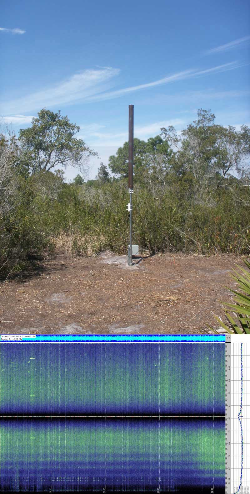
All the above spectrograms are of the “Schumann background” or the quasi-permanent SR field oscillations. Modes above 40Hz are usually very difficult to see as they are buried in the “Schumann background” spectra, because the corresponding wavelength is generally several thousand km and multiple sources are non-coherent at this spatial scale (source). Every so often though spatially isolated gigantic discharges can excite the Earth-ionosphere resonator in such a strong manner that the higher modes can be distinguished in spectra obtained from short time series (a few seconds). Below is an example of a Q-burst taken at my location. The frequency range is from 0Hz to 120Hz and the time period is about two seconds (time is EST). This Q-burst was captured with a new and much improved ELF receiver which I installed with the help of Brian Miller at Electricterra. Here is an image of the new setup with a spectrogram showing the first seven SR modes.

Many Q-bursts are characterized by a “double-spike” like pattern and their amplitudes exceed in most cases the average “Schumann background” by a factor of 10 to 20. It’s the huge size of these discharges that allow the higher modes of the SR to be observed in short time series spectra. Below is the frequency domain plot for the same above Q-burst. The first seven modes are clearly visible before the analog 60Hz notch filter begins to take over. On the upper side of the notch filter numerous higher modes which usually are non-existent become clearly visible.

The leading bipolar spike in the “double-spike” pattern of Q-bursts (time domain example above) is caused by the lightning discharge directly. The second spike is actually the around the world signal as it reaches the receiver! This delayed spike is usually slightly attenuated and widened in time due to dispersion. The time interval between the two spikes is in the order of 130-160ms and corresponds to the wave front travel time for one Earth orbit.

Research has shown that there is a strong link between sprite generating lightning and Q-bursts. On the evening of March 26th, 2010 I was able to image a number of sprites over the Gulf of Mexico which exhibited strong ELF transients. Here is an example of one such sprite. There were clouds in the field of view hence the fuzzy sprite.

The above sprite was caused by a strong lightning which generated a Q-burst that was captured by the ELF receiver. In the below plot the sprite generating Q-burst is the second larger transient. The characteristic “double spike” pattern of many Q-bursts can be seen in this transient and is labeled “Double Spike”. The delay between the first and second spike here is around 160ms. Not all sprite generating Q-bursts possess this double spike pattern. From my observations about half of all sprite generating Q-bursts show the double spike pattern.

Here is another example of a bright sprite caused by a Q-burst generating lightning captured on July 11, 2010. This sprite was extremely bright and much detail can be seen within the sprite including bright tendrils and a diffused upper region. This was pointing north over Georgia.

Here is the accompanying Q-burst for the above sprite. As can be seen this transient is huge compared to the surrounding activity. The “double spike” pattern is clearly seen in this Q-burst as well. The delay between the first and second spike for this one is again around 160ms. Damped oscillations after the initial spike and before the second spike are also visible. This was clearly a bell ringer!

I have forwarded some of these Q-burst “double spike” examples to a few academics and interest in them has been shown. I was asked by them to create a histogram of delay times between the “doublets” (as they termed them). Subsequently I began taking measurements for a two week period during March 2010 and below are the results. This histogram consists of a little over one-thousand Q-burst samples. Delay times run along the ‘X’ axis and Q-burst counts along the ‘Y’ axis. The histogram shows three “spikes”; a large one at around 150ms, a smaller one at around 130ms and a much smaller one at around 110ms. I find these delay times intriguing! My interpretation of the delays is that the large spike at 150ms is from Q-bursts originating in the Amazon basin (for the most part). The smaller at 130ms is from Q-bursts originating in Africa (the Congo region), and the smallest at 110ms is from Q-bursts originating in maritime south-east Asia. If one thinks about this logically it sort of makes sense. One would expect the largest delay times to be from nearby Q-bursts since the delay time between the first and second spike (round-the-world wave) would be longest with nearby Q-bursts. I have evidence that this is indeed correct from actual sprite generating Q-bursts which I have imaged and recorded (example above). I have yet to measure delay times below 155ms for sprite generating Q-bursts showing the “double spike” pattern.

One possible use for Q-bursts is as a proxy for global scale sprite detection. The problem with this is that it has been shown that not all Q-bursts generate sprites, so obviously there are other factors at work in sprite generation. Regardless, monitoring for Q-bursts is but one more fascinating aspect of Schumann resonance study.

Thanks for reading, and please email me if you have any questions.