Sudden Ionosphere disturbances (SID) are caused in large part by UV and X-ray generating solar flares. Solar flares occur when sunspots with very complex magnetic fields become unstable and explode. The X-ray and UV energy released by these solar flares makes its way to Earth and interacts with the upper atmosphere to create a SID. Therefore, one could deduce that if a SID device could be built to monitor radio stations which rely on the Ionosphere for propagation it could be possible to “indirectly” detect solar events. Well, it just so happens that this approach is a very effective way of detecting X-ray generating solar flares. It’s even possible to detect Gamma Ray Bursts (GRB) with these receivers believe it or not.

First though, an explanation of why a SID occurs in the first place is needed. SID receivers are built to operate in the VLF range. This frequency range is from 3-30KHz and possesses a number of unique characteristics. VLF signals are capable of traveling as powerful wave fronts which follow a trough formed between the Earth’s surface and the Ionosphere. These signals are able to travel large distances and I have monitored NWC in North West Cape, Australia from my location here in Florida a number of times in the past. VLF signals follow the curvature of the Earths crust and can also penetrate a ways into the crust. This is why the United States and other countries operate VLF stations. These stations are used to communicate with submerged submarines.
Now, SIDs come into the picture with the fact that VLF signals are capable of being reflected from the Ionosphere due to the creation of a wave guide between the Earth’s surface and the D layer. It is this wave guide and the various electron density variations that are present in the D layer and E layer that cause the variations in signal strength we see in SID receiver plots. During quiet solar days the D layer is more or less in equilibrium, but when there is a solar flare event the extra energy impacting the Ionosphere serves as an additional ionizing source which causes an increase in the density of free electrons throughout the D layer. The increase in free electrons makes the D layer a better reflector to VLF signals and also lowers it’s height. The end result is a significantly stronger VLF signal thanks to the sudden ionosphere disturbance.
I have for some time been interested in building a SID receiver to monitor solar activity. I first tried using an HF receiver and a VLF converter to do the job, but because the receiver had no way of turning off the AGC (Automatic Gain Control) I was not able to detect any SID activity. I was able to detect the daily pattern in the VLF signal strength though, so that did give me hope. I then decided to just build a simple SID receiver from scratch. The place to go for all your SID needs really is AAVSO. Those guys have their stuff together and is where I got most of my SID information from. I initially experimented with the “Simple, Easy-to-Build, SID Receiver“, but after some use I decided to build a better receiver. I had built a four foot plus diameter square loop for my natural radio receiver which I wasn’t using any longer. This loop is much larger than the small indoor loop I was using for the “Simple, Easy-to-Build, SID Receiver” and fit the bill for an outdoor SID receiver perfectly.

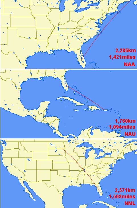
For the new receiver I decided to go with Renato’s Easy VLF Loop design. This receiver isn’t designed to be a SID receiver per say so I had to add some extra stages to make it work for my purposes. The stations which I monitor fall above 24KHz (NAA 24KHz, NML 25.2KHz, NAU 40.7KHz), therefore I added two extra OP27 gain stages behind the Easy Loop circuit to increase the gain in my working frequency range and to add filtering. I added a total of six RC filters, three low pass and three high pass. The purpose of these filters was to create a band pass filter with a low cutoff around 10KHz and a high cutoff around 47KHz. This allowed for the high amplification of the signals I wanted to monitor while at the same time limiting power line noise.
As this is an outdoor receiver there has to be a way for feeding the signal into the house. For the feed line I used about 200 feet of Cat5 cable and balanced the feed pair using two 1:1 isolation transformers between the preamp output and soundcard input. The circuit is powered via a pair in the Cat5 cable which feeds 12V from the house to the receiver. Another reason for the high amplification at the preamp side was to ensure that plenty of signal reached the soundcard due to this long run.
This receiver doesn’t have selectability past the band pass filter and it doesn’t demodulate any of the VLF signals. Due to this software has to be used to complete the SID station. I use Spectrum Lab by DL4YHF and a SoundBlaster X-Fi (96K sample rate) soundcard for this purpose. Within SpectrumLab I use the “Plot Window” and the peak amplitude expression to monitor all three VLF stations for amplitude variations in real time. Using software to monitor for SID events has many advantages and the ability to monitor numerous stations at once is by far my favorite.
This completes the SID monitoring station. The monitoring station consist of the large loop antenna, the three stage OpAmp amplifier/filter, the feed line, and the soundcard/software used for unattended monitoring. So what can you expect to see on a quiet solar day? Well, below is a set of plots during a typical quiet solar period.

The plots start at around 2:00 a.m. local time here in Florida (EST). During nighttime hours the VLF signals drastically increase in signal strength and then begin to vary due to fading. Presumably the propagation path during these hours is via the E layer. These are the hours where the receiver is not capable of detecting SID events from solar flares. After all, the Sun is on the opposite side of the planet. Between 6:00 & 7:00 a.m. local time the signals begin to drop in strength. This is the transition between E layer sky wave propagation and D layer creation/propagation due to the Sun’s ionizing effect on the Ionosphere. During daylight hours and quiet solar periods the plots will be pretty close to a straight line. This is because during these hours the D layer is more or less at equilibrium. Now, if there was a solar flare of sufficient size during the daylight hours, like the example below, the plot would show a sharp rise (or drop) in the signal strength of the VLF station and then a slow decay back down to the previous level. It’s possible to tell how strong the solar flare was just by looking at how much the signal increased before going back down again. The three VLF tations monitored are at different distances from the receiver so the dawn/dusk patterns are different for all three. I find it interesting to study these variations on a daily basis. Here is a great circle map for each of the paths with the distances labeled.
Now here is an example of a somewhat active solar day. On Dec 18, 2009 at 1855UTC a C5 solar flare from sunspot 1035 erupted causing a SID event on the below plot. Since the flare occurred later in the afternoon (Florida), the NAA and NAU paths showed small variations where the NML path which was still well lit by the Sun showed a much more pronounced spike.

I should again stress that this is a very effective way of monitoring the Sun for solar flares, and many Universities and scientist use this technique as a supplement to the more advanced techniques such as satellite monitoring of the Sun. Furthermore, SID event monitoring is used by scientist to study the D layer itself. The electron densities in the D layer are not high enough (typically < 10^3 cm^-3) to allow ionosondes and incoherent scatter radars of even the highest power to receive significant echoes from this layer. Also, the D layer is too low in altitude for conventional satellites to make in situ measurements yet too high for balloons. Therefore, the D layer is very difficult to study by scientist. SID monitoring is one effective way of studying this poorly understood layer of the Ionosphere.
Solar flares not only generate energy in the X-ray bands and above, but all the way down to radio waves. Another effective way of monitoring for flares is with HF receivers tuned to the 21MHz frequency range. Here is an example of a C6.6 flare recorded using my Icom 751 HF transceiver: C6.6_Flare_02142011_1930UTC. The actual recording is around four minutes long, but I shrunk the file to make the radio burst more obvious.
Lightning-induced Electron Precipitation
With a sensitive SID receiver it is possible to monitor other ionosphere phenomena besides solar flare induced disturbances. Lightning-induced electron precipitation (LEP) is one such phenomena that I find fascinating. LEP events occur when strong lightning strikes couple some of their energy through the ionosphere into the magnetosphere. Once in this realm the energy is termed “whistler-mode wave” and is the subject of my Natural Radio page. Whistler-mode waves can be of two types, “ducted” or “nonducted”. In the ducted case the whistler wave can be detected in the opposite hemisphere as a falling tone. In the nonducted case the whistler wave is not trapped within field-aligned ducts and instead propagates obliquely through the medium. Most whistler mode waves are of the nonducted type (we never hear them on the ground only from space). Both of these whistler-mode wave types interact with trapped radiation belt electrons via cyclotron resonance, leading to pitch angle scattering of the electrons, causing some of those close to the loss cone to precipitate into the lower ionosphere where they produce secondary ionization. It is this secondary ionization that can be indirectly detected by monitoring VLF stations.
For detecting LEP events a faster sample rate is needed than when monitoring for solar flare events. In my case I sample at about 11 samples per second. This allows for the detection of these much “faster” disturbances. A typical LEP event will have a fast onset curve (up or down) in the order of a second or so. In many cases the causative lightning can be seen on the plot preceding the onset by about one second. Then there is a recovery period back to the previous signal level of between 10s and 100s. These variations are in the order of a few dB so they are small! The effect of this is to make the plot look like a “ramp”. LEP events occur poleward of the causative lightning by 2 to 6 degrees or so for lower latitude stations (dependent on the cold plasmaspheric density profile). Therefore one should look for VLF propagation paths having strong storms to their south for possible LEP activity.
Here is an example of a LEP event taken on September 18, 2009 at 0143 UTC. The LEP occurred on the yellow line, NML path. The green and blue lines are NAA and NAU. The red line is the noise level. The sample rate was set to eleven per second, and the time ticks were every ten seconds. The recovery time seems to have been around 10 seconds. Click on the image for a higher resolution version. Here is the audio for the below spectrogram. The strong tweek towards the middle of the sample corresponds to the “Source” labeled on the spectrogram.

Early/Fast Events
Another lightening induced ionosphere phenomena that can be detected with a SID receiver is early/fast events. Early/fast events differ from LEP events in that the ionospheric disturbance that causes the VLF signal to change strength or phase is caused by direct heating or ionizing of the ionsophere by the lighting strike. As can be seen this is a totally different mechanism than that for LEP events. Early/fast events are called such because the causative lightning and the subionospheric VLF signal change occur simultaneously (<20ms). In LEP events the time between the two events is around 1 second.
I enjoy early/fast event monitoring because with this type of ionospheric disturbance one actually has the opportunity to photograph the phenomena that causes it. I am speaking of sprites. Sprites are large electrical discharges that occur high above energetic thunderstorms and they are triggered by positive lightning strikes within these storms. By using low light cameras it’s possible to image these transient luminous events or TLEs.
Following is an example of an early/fast event and the sprite which caused it. The event occurred on Oct 16th at 0750 UTC. Here is the image of the sprite taken with my Watec 902H and a 16mm f1.4 lens. The storm that generated this sprite was 250 miles to the northeast of my location and directly in the great circle path (GCP) for NAA.
![]()

Due to the storms location within the GCP of NAA and my location, the above sprite was able to disturb the ionosphere and cause the dip on the green plot line (top line) below. The yellow plot line is NML and the blue plot line is NAU. The positive lighting which caused this early/fast event can clearly be seen as the spike on all three transmitter plot lines as well as the noise line (red). The signal level for NAA took about 10 seconds to recover back to it’s previous level which is typical for these events. Here is another example of an Early/Fast event which occurred on the NAA path. The sky was overcast on this night so I have no accompanying sprite for this event.
![]()
The above plot lines give a rough view of the amplitude of each VLF transmitter. Only the stronger early/fast events show up when using this technique. Thankfully Spectrum Lab by DL4YHF
Hi, could you supply a schematic for the SID receiver?
Hello, for the SID receiver I used a simple H field OP-Amp receiver. I followed Renato’s Easy Loop design.