One of my many interests is HF propagation study. For years I’ve wanted to study HF propagation by monitoring broadcast station signals on the HF band. The challenge with this sort of work is that very stable receivers are needed since one has to “zoom” in on the signal down to say 2.5Hz to either side of the carrier signal of the broadcast station! If a very stable receiver is not used (in the range of 1ppm drift or better) then the carrier being monitored will simply drift right out of the pass-band of the monitor software. Therefore, that puts all receivers that don’t use at least a TCXO (temperature controlled crystal oscillator) out of the question. With that said, things have come a long way since I first became interested in this subject. Today we can capture reasonably stable HF dopplergrams with a SDR that cost $20!
For an excellent explanation and background regarding HF propagation and dopplergrams please visit ZL1BPU’s site.
I’ve been experimenting with HF Doppler using an RTL-SDR Blug V3 which has a TCXO in place of the less stable crystals which these cheap units normally use. I’ve been pleasantly surprised with the frequency stability of this unit! It has allowed me to do interesting experiments related to HF propagation. Following are some examples with explanations of what you can expect to capture with a similar setup.
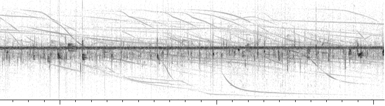
This example is of WWV on 10MHz using a 5 Hz width setting centered on the carrier. WWV is 1,700km from my location (Tennessee) and at 10MHz the propagation is at a lower angle and 100% via the F layer since the E layer isn’t typically ionized enough to reflect signals at these higher frequencies. The times are local and sunset is around 1720. The variations on the carrier are caused by the F layer reflection points oscillating up and down and causing a Doppler shift up or down in frequency depending on the direction of movement. You can also see two distinct lines in the plot and these are the right-hand and left-hand circularly polarized signals or ordinary and extra-ordinary rays. About 40 minutes after sunset the ionization level starts to drop closer past the levels needed to cause reflection and you start to see both the low path and high path ray (Pedersen ray). As ionization keeps dropping the two rays get closer until they meet at the ‘nose’ of the dopplergram and you get skip fadout and the band closes! Ham radio operators are very familiar with this phenomena and the response is to spin the radio dial down in frequency to the next lower Ham band to continue operations.

This is a morning dopplergram of CHU on 7.850MHz at around 1,450km distant. As expected, there is a fold-back pattern similar to the evening example above, but in the morning the pattern is flipped and the fold-back occurs on the high frequency side. The E layer is clearly visible as it becomes ionized and begins playing a role in propagation at around dawn local time. The fact that we can differentiate between E layer and F layer propagation in this dopplergram is fascinating to me. Not only can we tell the difference, but we can also tell what mode of propagation is occurring at any one time. For example, we can see that initially we have direct ray propagation from the F layer (well defined line) and then it changes to F layer scatter.

Here is another example, this time monitoring WWV on 5MHz. The times are local and sunrise is around 0630. At 5MHz the E-Layer is involved in propagation during the daylight hours and can be seen on the dopplergram starting at around dawn. F-Layer scatter coming down from the high frequency side at around dawn is also visible as the F-Layer starts to give out due to D layer absorption and by 1000 only E-Layer propagation is visible.

Now this example is the main reason why I wanted to experiment with HF dopplergrams. This is an example of ocean wave Bragg scattering off the Atlantic from WEWN on 15.610MHz. WEWN is only about 150 miles from my location so on the higher frequencies I’m well inside the skip zone of the station. During the day WEWN broadcasts on 15.610MHz beaming first to EU at 40 degrees and then Africa at 85 degrees. It’s a perfect setup to watch how the signal backscatters off the northeast US landmass as well as the Atlantic ocean during the 40 degree broadcast and then only from the Atlantic ocean during the 85 degree broadcast.
On this dopplergram you can see that while its beaming 40deg you see the center trace which is backscatter from a landmass. Then on either side you see two more traces which is Bragg scattering from the Atlantic off the side of the beam. The sidebands are .40Hz to either side of the center signal. The formula to get the spacing of the sidebands is Hz = 0.1*sqrt(MHz).
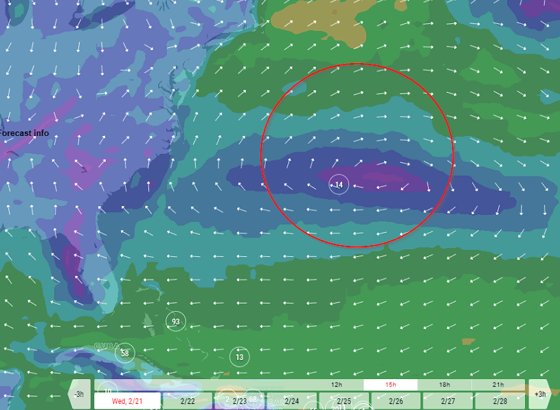
So here is the cool part! When WEWN switches to 85 degrees, the landmass backscatter goes away and you are left with just the Bragg scatter which is being reflected back from somewhere out in the Atlantic. From observations of wave direction patterns it looks like the reflection area is near Bermuda for my particular setup. So if the waves in that area are predominantly moving towards me we should get a stronger upper sideband and weaker lower sideband. If the waves are mostly moving away we should see a stronger lower sideband. In this example there was an area of high pressure that was causing the waves to go both towards and away from me in the reflection area so both sidebands are really close in intensity. Check out the wind map, the red circle is where I think the backscatter is originating from.

Here is an example of the lower Bragg sideband reflecting stronger due to the predominant wave direction moving away from my station in the reflection area. The slight variations in the signal frequency in the plots is receiver drift due to temperature variations (AC turning on and off). Therefore, this is the level of stability expected from this particular SDR unit. It’s good, but it could be a lot better.

An example of Bragg Scattering in the frequency domain.

Finally, this technique can be used as a sort of CW Doppler radar. On the below plot all the long traces above and below the carrier are aircraft. You will want to tune into a shortwave station that is near your receiver. Within 100 miles or so should do. As aircraft come in range of the “radar” they reflect some of the signal and it shows up on the plots as Doppler traces first with a high frequency Doppler shift and then a lower frequency Doppler shift as the aircraft passes by. This is a similar effect as when an ambulance passes by and the siren is higher in pitch as it nears you and then lower in pitch as it passes by. One can also calculate the speed of the aircraft by taking the Doppler shift observed and multiplying it by the half wavelength of the monitored frequency. In addition meteors can be monitored with this same technique and can be seen on the below plot as the vertical “squiggly” lines. These are meteor Doppler trails!

Another way to study the Ionosphere is via ionospheric sounders. Again, with the advent of SDRs and Internet SDRs in particular we are now able to carry out experiments that 10 years ago would have been very difficult to do. Below is an example of one such experiment. This is a scattergram of a Stanag 4285 British NATO transmitter. Peter Martinez, G3PLX is the expert in this field and all the above dopplergrams and below scattergrams were taken using his amazing software.
So what are we looking at here? Well, in the center bottom of the scattergram is a round white dot. This is the groundwave signal from the transmitter. The software locks onto this ground wave and does all subsequent calculations of delay and doppler shift in respect to this ground wave signal. Along the horizontal axis is frequency +/-4.6Hz and vertically is time delay from 0ms to 13ms. For the software to work properly you have to be within ground wave range of one of these Stanag 4285 transmitters, hence my comment about Internet SDRs like the Kiwi network of GPS synchronized receivers. If the stars align and you are within ground wave of one of these stations or find a Kiwi SDR within range then you are able to experiment with Near Vertical Incidence Skywave (NVIS) phenomena, both skywave and groundwave ocean wave Bragg scattering, ranging of NVIS and backscatter signals, monitoring field aligned backscatter (aurora backscatter), aircraft detection, meteor detection and more.
In this scattergram taken at 5Mhz on one early August British evening you see the NVIS signal reflection from the F-layer just above and to the right of the center dot with 2 hop, 3 hop, 4 hop and 5 hop NVIS F-layer reflections above and drifting slightly to the right of the main F-layer return. For a portion of the clip you can also see a dot which corresponds to the E-layer just above and to the left of the center dot. This might have been a meteor from the Perseid meteor shower that was ongoing during the capture. Aircraft look like small dots crossing from right to left along the very bottom of the scattergram. This clip has no aircrafts in it. In this example the F-layer is at around 2ms delay or so which puts it around 300km up. The E-layer is around .6ms delay which puts it at around 90km above the receiver. As you can see this is a very capable tool for HF propagation studies.

This noted scattergram should help clarify things.

Here is another great example of what is possible using the scattergram feature. In this example the signal was from the Stanag 4285 station PBC in Netherlands on 8408.2Khz. In this scattergram we can see a number of features.
A: Groundwave Bragg backscatter. Dot seen .29Hz above the main carrier. This tells us that the predominant wave direction is onshore near the shoreline of the Netherlands.
B & C: E-Layer Bragg backscatter. This is Bragg backcatter off the E-Layer with a 3.5ms delay or so. We can clearly see a low frequency and high frequency sideband (+-.29Hz) which tells us that the wave direction is either in multiple directions or perpendicular to the shoreline. In addition since the delay is 3.5ms this tells us that the reflection point is some 525km off shore. In this case most likely somewhere in the middle of the North Sea.
D: F-Layer backscatter. This fuzzy looking area is F-layer backscatter and the delay puts the reflection point past 900km.

An example of how aircraft look on the scattergram. F-Layer backcatter and groundwave Bragg backcatter are evident as well.

Another good example of aircraft trails

While not HF per se, here is another fun way of experimenting with Doppler. I’ve been experimenting with monitoring the GRAVES (Grand Réseau Adapté à la Veille Spatiale) French radar-based space surveillance system operating on 143.050Mhz. I use the CAMRAS web SDR in the Netherlands for the task. Here is an example of what to expect with the setup. The center vertical line is from aircraft reflections having small Doppler shifts. The vertical dotted line to the right (high frequency) of the center line is actually the Moon reflection from the transmitter. It’s high frequency in this example because the Moon was to the East of the transmitter, that is approaching the transmitter. As the Moon nears the meridian the Doppler shift decreases until it becomes zero. The sloping line going from right to left is the ISS as it passed over the Mediterranean. The huge Doppler shift difference when compared to the aircraft traces near the center of the screen gives us an idea of the speed the ISS is traveling at! Meteors are also easily detected with this setup as with the HF approach above.

Hope you enjoyed the post and happy experimenting!

Nils Schiffhauer
Thanks, excellent combination of theory and practice! I also observed the Bragg reflection of 1st and 2nd order, latter plusminus 0.1 Hz from RFI Issoudun 15300 kHz from the Alboran Sea/West Mediterranean Sea, near Hannover, North Germany. Did you ever received Doppler of Longpath reception thanks to the rotation of earth? 73 Nils, DK8OK
w4gon79
Hi Nils, I haven’t done any work with Doppler of long path signals. I’ve concentrated on backscatter signals only. I’d be interested to hear your findings if you have done any work in that area. Joel
John Gilbert
Excellent information very well presented.